At Modash, we need to process socials data at a petabytes scale to serve our customers - and this massive volume of data processing adds up on our cloud bills, time-to-market, and operational efficiency. With scale at this level, the data processing can no longer be done with a single node compute. Similar to the vast majority of organizations in the industry, we’re relying on Apache Spark to run our distributed data processing jobs.

Apache Spark is tricky to optimize, and most organizations treat it as a black box. Optimizing Spark jobs requires solid understanding of Spark’s architecture, execution models, and constraints — which provides clear view on the true bottlenecks. This article outlines the principles of Spark, followed by optimization levers that could help you and your organization saves a lot of money and time.

So, off we go to the principles that we applied during our optimization journey; bringing down processing costs by ~63% and execution time by ~76%.

Anatomy of Spark

Before stepping into the optimization tricks, let’s start with the structure of Spark.

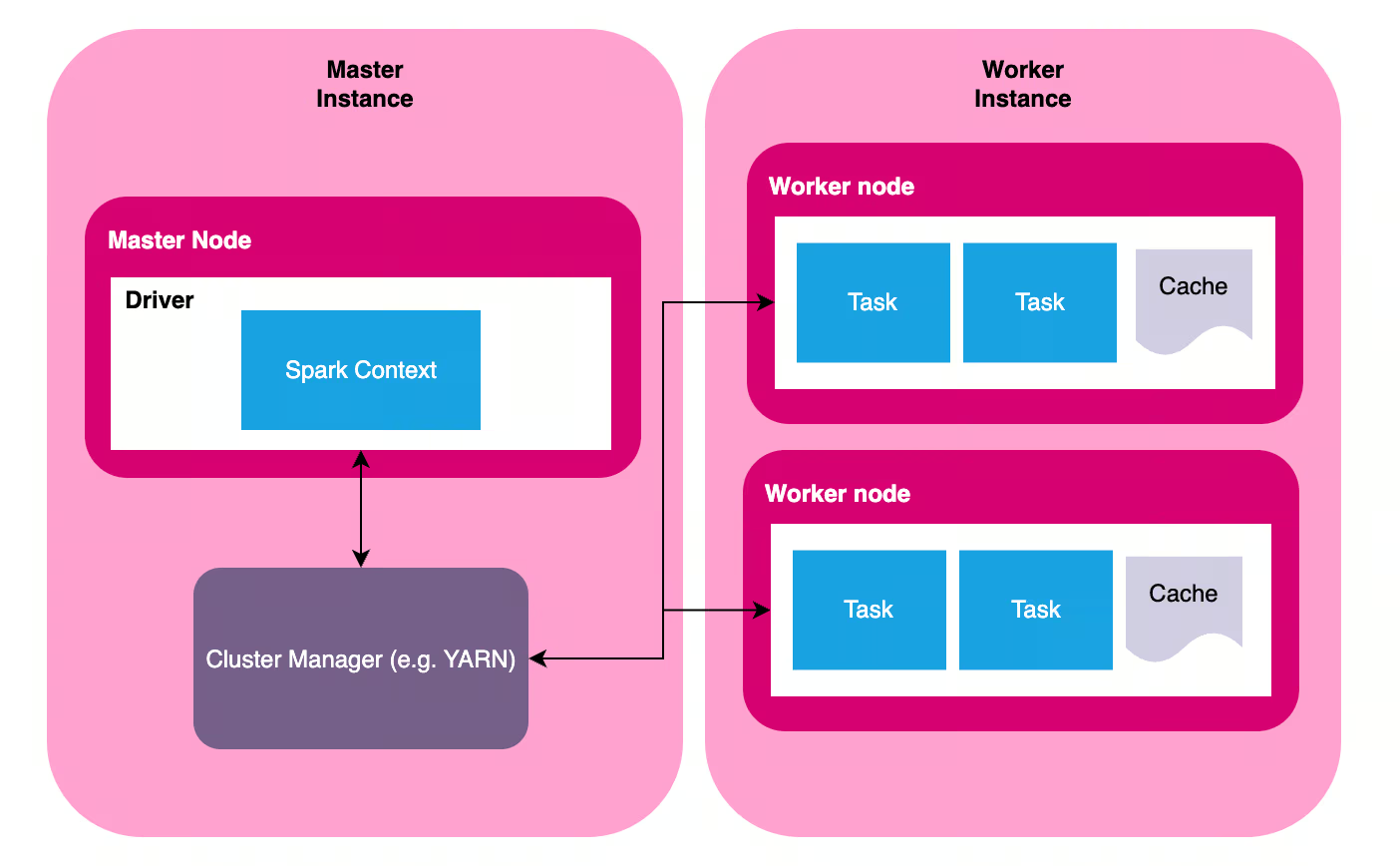
Spark is a distributed data processing tool, and as the name suggests, it consists of multiple instances that makes up a Spark cluster. A Spark cluster has one instance of master node (commonly called driver node) and multiple instances of worker nodes (also called executors). Each node might be running in separate physical computers, or a virtual instances running in the same computer.

• Master node is responsible for planning the job and managing the execution. Job planning ranges from generating physical query plans based on logical instructions (SQL/PySpark/Spark script), selecting a plan, translating this plan into execution stages, and generating tasks for each worker. Execution management involves distributing tasks to worker nodes and ensure tasks are processed successfully; includes retrying stages/tasks if necessary. There are many terminologies here (query plan, stage, task), and we’ll get to it in the next section.
• Worker node is responsible for the actual data processing based on the task assigned by the driver node.

Spark was first built in 2009 - in an era when computing infrastructure wasn’t that stable. Thus, the tool was built with fault-tolerance baked in. Even if some worker nodes fail in the middle of the process, or even if some of the physical computers crashes, the show must go on. Spark’s master node communicates with a cluster manager (for example, YARN or Kuberneted) to check the health of the computers in that cluster, and dynamically adjust the cluster to get the job done - from killing unresponsive nodes, spawning new workers, or even killing the whole job if there is no available resource to finish the job successfully.

It’s important to keep the distributed nature in mind, as it’s the main principle we’ll rely on when optimizing a Spark job.

From Logical Queries to Physical Plans

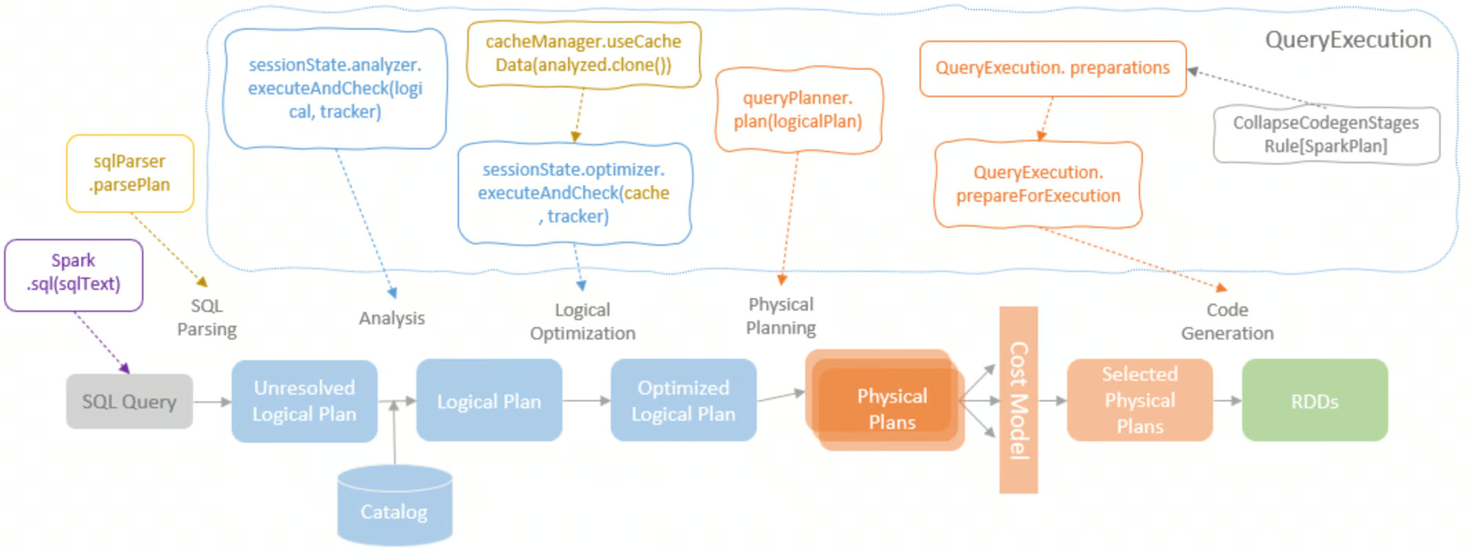
In Spark, what you write is not what you get. The Spark script (for simplicity, we’ll use the term logical plan to refer to this) is not an explicit instructions of how Spark should execute the computation, it’s simply a description of the computation. Based on this description, Spark will translate this logical plan into physical plans.

Physical plan represents the actual physical operations that will take place to carry out the calculations defined in the script. For each logical plan, Spark generates different options of physical plans — and choose one plan to be executed.

The physical plan is represented by a Directed Acyclic Graph (DAG), a map of every computation step and how they depend on each other. For example, look at a simple SQL query below and the corresponding plan (and the DAG).‍

-- Logical Plan
SELECT COUNT(*) FROM table
-- Physical Plan
AdaptiveSparkPlan (isFinalPlan=false)
+- HashAggregate
	+- Exchange SinglePartition
		+- HashAggregate
			+- FileScan parquet orders

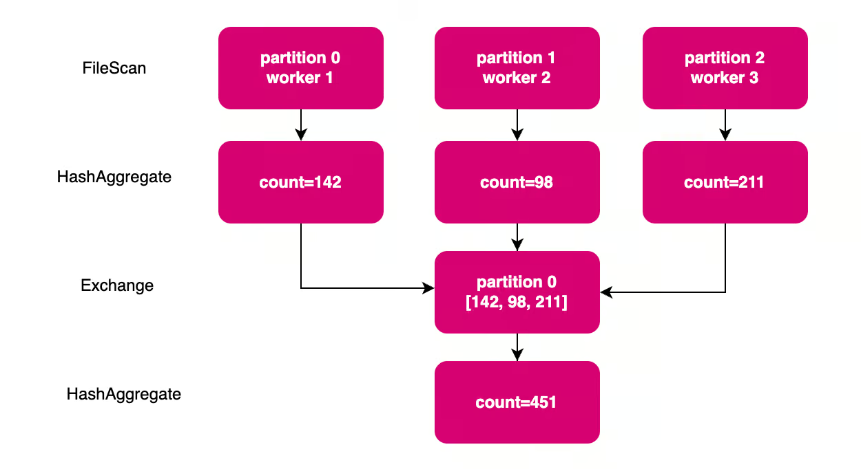
In the example above, a simple logical plan (SELECT COUNT(*) … ) is translated into a series of physical operations.

The first operation is scanning the data and loading them into memory (FileScan). This data loading is executed by each worker nodes, each only loads a subset of data. Then, each worker calculates the partial aggregate in each nodes (the first HashAggregate), followed by shuffle (Exchange). A shuffle represents data redistribution between worker nodes. In this example, each partial count calculated by each node needs to be collected into a single step to get the final count.

Lazy Evaluation Model

Spark applies a lazy evaluation model, which means the cluster will only do work when it has to. The instructions defined in the script (like joining two datasets, aggregating values, or filtering on a condition) don’t actually trigger computation. Only when an action is triggered (like writing the output to disk, or collecting the result to the master node), then Spark starts generating the execution DAG based on the aforementioned instructions.

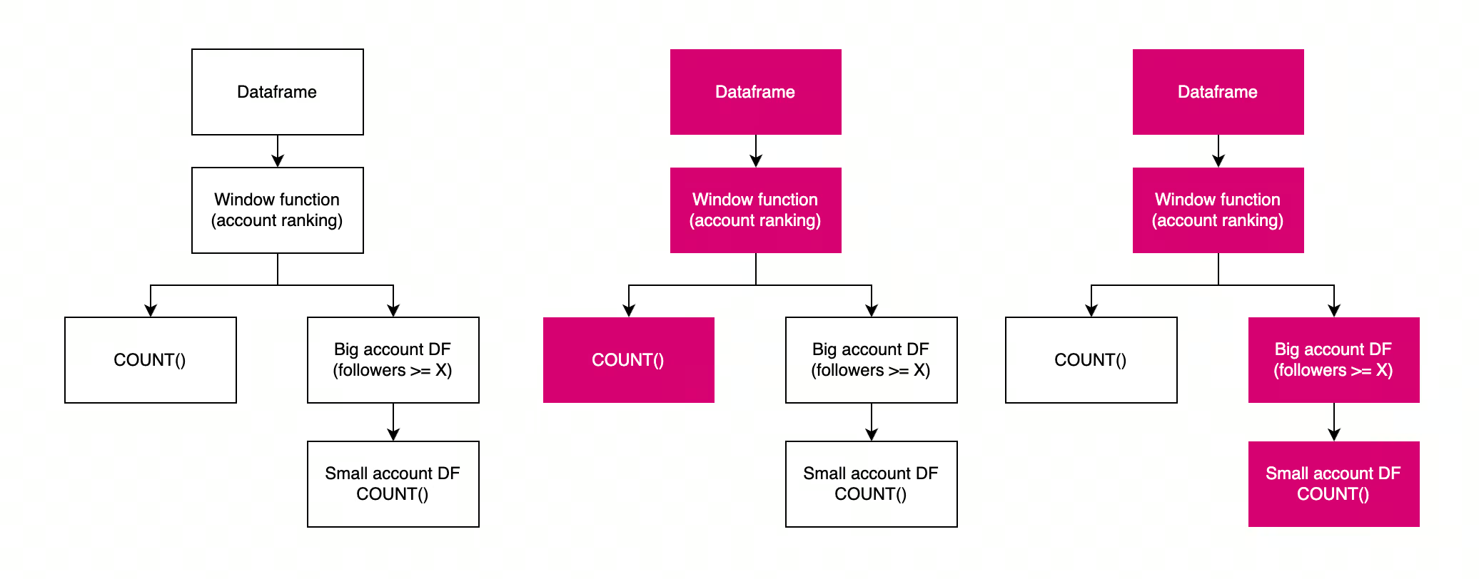
This lazy evaluation model sometimes is responsible for poor job performance; not from an actual heavy load of data processing, but simply for repeated calculations triggered by different actions. The diagram below shows an example of repeated calculations from poorly-scoped action calls.‍

df = spark.read.parquet("s3://bucket/users")

window = Window.partitionBy("category").orderBy(F.desc("followers"))
df = df.withColumn("rank", F.row_number().over(window))

row_count = df.filter(F.col("rank") == 1).count()
logger.info(f "{row_count} rows after ranking") # Action 1

df = df.filter(F.col("followers") > 1000)

row_count = df.filter(F.col("rank") == 1).count()
logger.info(f "{row_count} rows after follower filter") # Action 2

‍


Stages & Tasks

One DAG represents one job for Spark. A job is broken down into multiple stages, separated by shuffle boundaries. Each stage is further divided into tasks, one task per one data partition. The tasks are the actual unit of work dispatched by master node and carried out by worker nodes.

Spark keeps track of the full lineage of the calculation, from the DAG, stages and tasks. This lineage helps Spark to be fault-tolerant without data replication: a failing task can simply be retried, and intermediate data loss can be recalculated by retrying the affected stages & tasks.

Compute, Memory, and Network Constraints

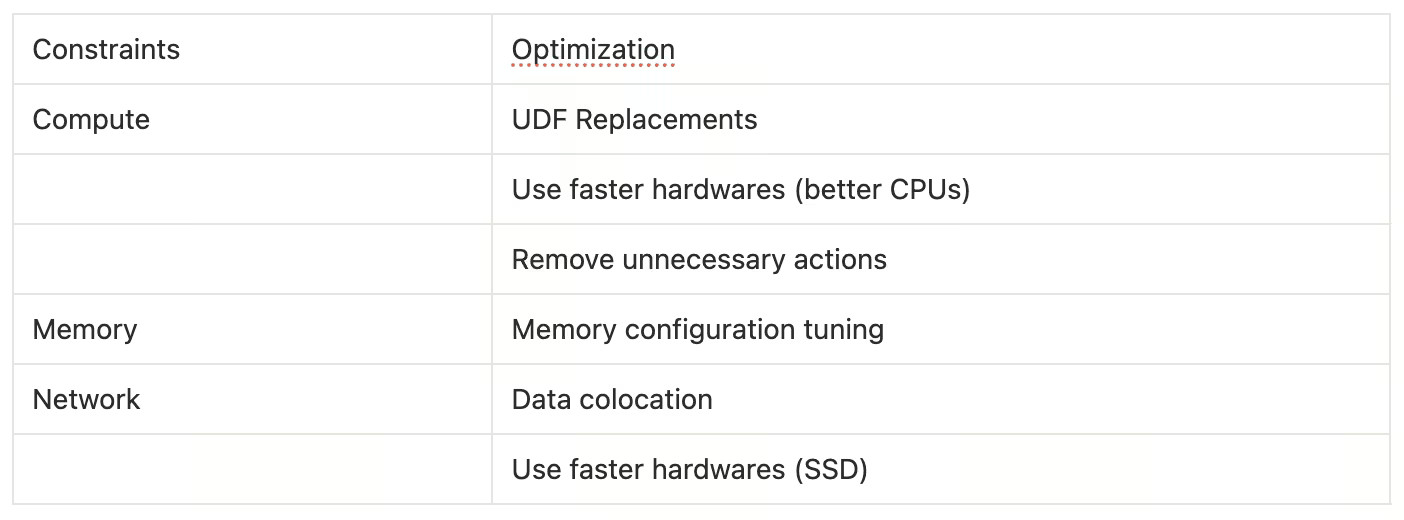
The sophisticated scaffolding of Spark makes it seems like a plug-and-play solution, but the tool is still constrained by physical limitations. At the end of the day, data processing means crunching 1s and 0s in the physical transistors, and there are physical limitations to each of the bottlenecks: (a) compute, (b) memory, and (c) network.

Compute: Limitations of CPU & JVM

It goes without saying that the speed of each execution cycle is constrained by the CPU’s capacity. However, some modern CPU supports parallelized calculation on the hardware level, such as SIMD (Single Instruction, Multiple Data) that offers parallel computing for each CPU cycle. However, vanilla Spark doesn’t take advantage of this.

Spark is written in Scala, and it runs on JVM (Java Virtual Machine). When you write a Spark script (whether in SQL, Scala, Java, or Python via PySpark), it gets compiled into bytecode - an intermediate representation that isn't specific to any particular computer architecture. This bytecode is then executed by the JVM, which acts as a translation layer between your script and the actual hardware.

This design allows Spark to run on any platform that has a JVM (Windows, Linux, Mac, etc.) without needing to rewrite the code for each system. However, this architecture-agnostic approach comes with a trade-off: the JVM abstraction layer prevents Spark from leveraging hardware-specific optimizations like SIMD instructions that modern CPUs offer for parallel computing.

Memory: Spill & OOM

Spark is designed to be an in-memory processing engine. It works the best when the data fits into memory. This in-memory paradigm is the main reason why Spark is magnitude faster than its predecessors, which uses disk-based storage.

However, in real life scenario, often times the data is bigger than what Spark can store in-memory. When this happens, the data is spilled into disk to free up some space in the memory. Spillage is a performance killer because writing to (and reading from) disk is slow. When spillage happens, the performance of your Spark job is also constrained by the disk I/O speed.

Another memory constraint is the bare capacity of the memory. When the data is simply too big, there is not enough space to store all the 1s and 0s - leading to Out of Memory Error (OOM).

Network: Shuffle

We have briefly talked about shuffle in different places in this article, but what is it?

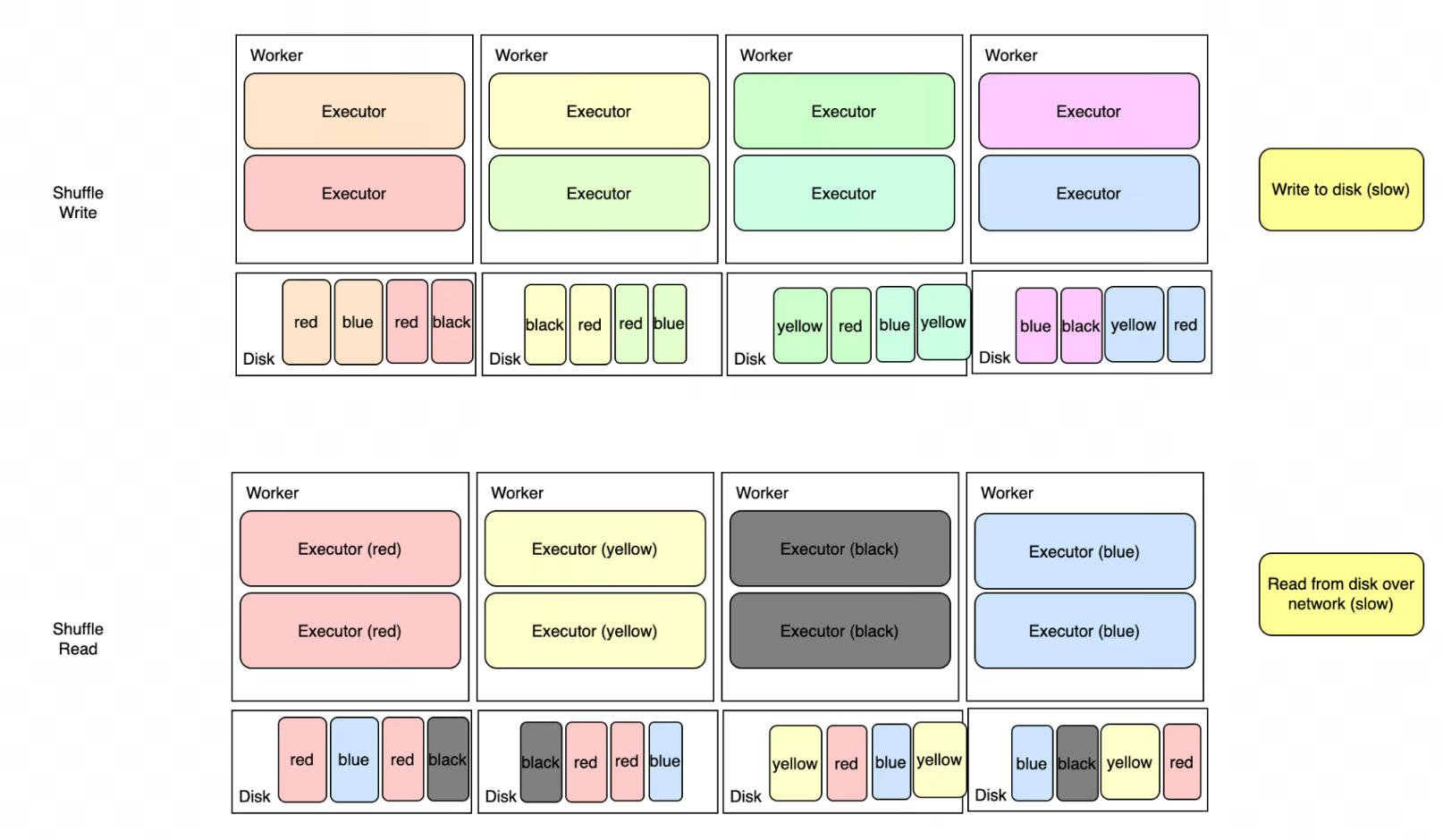
Shuffle (or referred to as Exchange in physical plan) is a data redistribution step between worker nodes. Some operations require data colocation (such as join, window function, or aggregations), and data colocation requires Spark to redistribute data around to guarantee this distribution requirement.

If you’re running SELECT country, SUM(gdp) from economic_data, all rows with the same country need to be physically located in the same worker node. Same thing with joining two datasets on a join key, or deduplicating rows based on a unique key.

In almost all of our pipelines, shuffle is the biggest culprit of poor job performance. Shuffle is a performance killer because of the slow multi-steps: (a) each worker writes data into disk, (b) each worker communicates with each other to read different slices of data, and (c) each worker reads data partitions from different nodes. It’s a disk I/O over network, and in cloud-based environment, there are no guarantee that worker nodes are located physically close to each other.

Optimization Tricks

Optimizing a Spark pipeline involves changing some parameters — be it changing the script, changing the storage layout, changing the hardware, or changing the configuration — to get around the physical constraints. In this blog, I’ll focus on vanilla optimizations that only rely on the vanilla Spark distribution.

There are so many knobs to turn, and this blog could be way longer than it should if we try to cover too many of them; so we’ll focus on a few tricks we implemented at Modash that has the biggest leverage to press the cost down.

Hardware Upgrades

The first step to achieve better performance is by upgrading the hardwares. We started using newer generation CPUs and use SSD-based disks. This is one of the no-brainer optimization without changing the job itself. SSD-based disk is particularly very helpful, as a lot of the slow parts of the job comes from disk I/O (read-write for shuffle & spill).

UDF Replacements

User-Defined Functions (UDF) are a common escape hatch in PySpark, but they carry a steep performance cost rooted in how Python and the JVM interact.

When a Python UDF runs, Spark serializes each row from the JVM to a Python process, applies the function, then deserializes the result back — one row at a time. Python UDF is extremely slow.

Ideally, Python UDFs need to be rewritten to use native Spark functions (F.when, F.regexp_extract, F.transform) or SparkSQL, but sometimes we depend on libraries in Python. In this case, migrating Python UDFs to Pandas UDFs already offers a significant improvement.

Pandas UDFs are faster because data transfer between JVM and Python is not done row-by-row, but batched into Arrow buffers and passed as Pandas Series. Pandas-based execution also benefits from the vectorized optimization, as opposed to strictly serial execution in Python UDFs.

The priority order when replacing a UDF should be:

• Native Spark function (F.when, F.regexp_extract, F.transform)
• Pandas UDF, if native cannot express the logic
• Python UDF, as a last resort only

Unnecessary Actions Removal

As described in the lazy evaluation section, we also gained performance improvements by simply removing unnecessary actions, like removing COUNT(*) in logs. If repeated action is unavoidable, the intermediate data can be cached/checkpointed to avoid recalculating the expensive upstream tasks.

In some cases, we reduced a 2.5 hours job into 30 minutes job by simply shaving the unnecessary actions!

Memory Configuration Tuning

Another trick is to adjust memory-related knobs. The goal is to reduce memory pressure, either by increasing memory per worker node, or by reducing the data size in each task.

• Bigger parallelism by increasing partition count. More partition count means less memory pressure per task.
• Increasing memory per worker node.
  • The easiest knob for this is by adjusting cluster configuration to use nodes with bigger RAM, and allocate more memory through Spark configs.
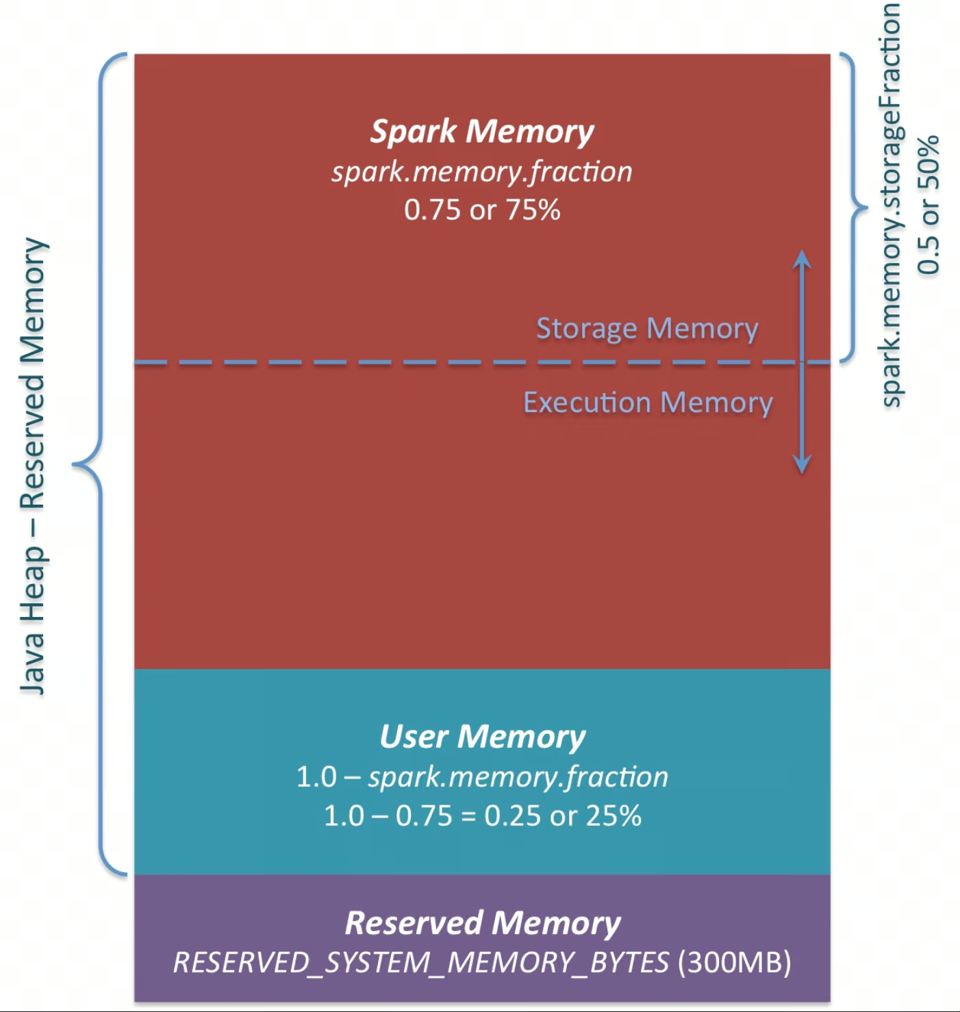
  • Another knob is to allocate more space in existing memory for workers. By default, out of all memory space — around 5-10% are reserved for OS & cluster manager. The remaining 90% are distributed for all workers in the same computer. These remainder are distributed between user memory and spark memory (configurable via spark.memory.fraction ). Spark memory is the space available for worker nodes, thus increasing this will give more memory for the workers to work with.
  • Aside from the overall Spark memory allocation, another config to adjust is spark.memory.storageFraction . The Spark memory space is further divided into two areas: storage & execution memory. Storage memory is used to store cached data; and it might not be strictly required in some cases. Reducing this space gives worker nodes more space to process data in-memory, which reduces spilling. However, keep in mind that reducing this space means less reserved memory for cache.

• Reduce GC pauses (JVM tuning)
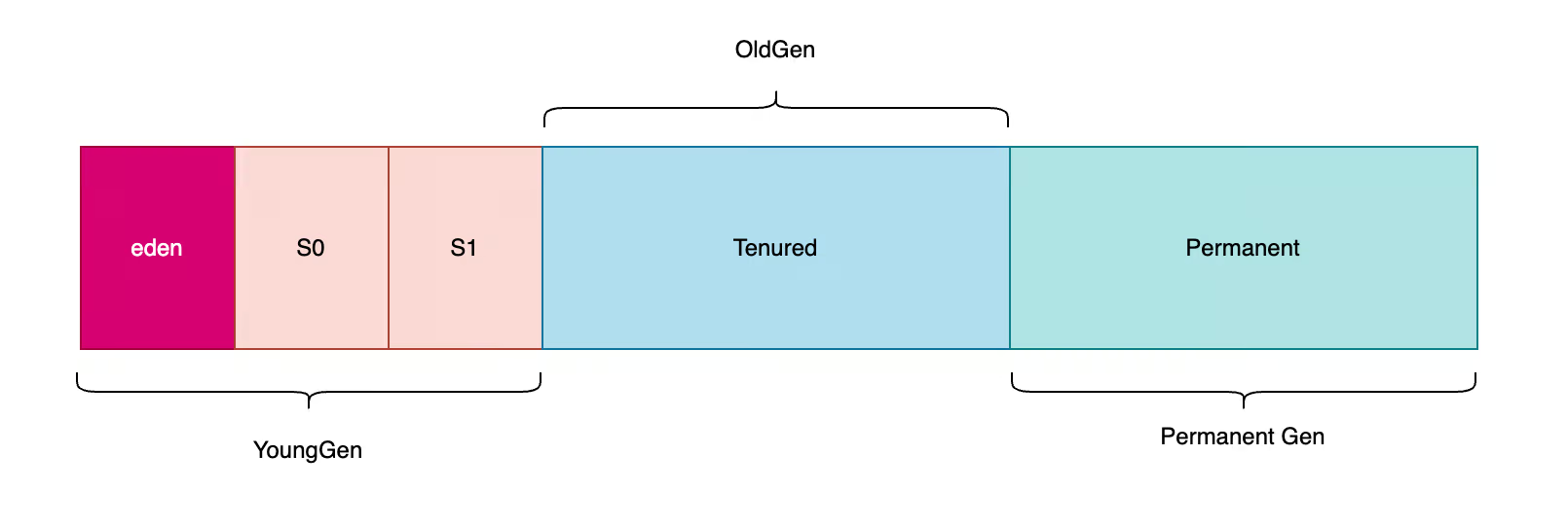
  • Spark runs on the JVM, so Garbage Collection (GC) can become a bottleneck in jobs with high allocation rates (e.g., heavy shuffles, wide aggregations, row-wise UDFs). Spark mainly stores data in memory inside a heap, and stale objects need to be cleaned via GC.
  • With the default GC setting, the heap is broadly managed as young (short-lived objects) and old (long-lived objects). Objects are initially stored in the Young region, and if it persists after some time, the said objects are promoted to Old region. Young-gen garbage collections are usually cheaper; frequent promotions and old-gen pressure can lead to longer pauses. When GC pause is triggered, Spark pauses its execution until the garbage collection is done. Frequent GC pauses could pile up and waste execution time. Optimization lever related to GC involves changing the GC strategy (from default to G1GC, for example), or adjusting the size of the regions. Keeping the Young-gen area bigger will give more space before GC collection, reducing time spent for GC pauses. Keep in mind that this lever is tricky to optimize and can be brittle, so careful experimentation is needed.

One important thing to note about memory tuning is the acknowledge the fact that it’s a brittle optimization, and it has to be contextual. Not all the configs will be applicable for all kinds of jobs. Try it out and evaluate the result before committing on a path!

Data Colocation

Last trick, and arguably the most impactful one, is to intelligently change the script and storage layout to achieve shuffle-less physical plans. If Spark can guarantee that the data are already distributed correctly, it won’t insert unnecessary shuffles.

Shuffles are inserted when operations require data colocation (related rows located in the same partition), and unless Spark’s optimizer have a guarantee that the data is indeed colocated, it will insert a shuffle step before the operation. Operations that require colocation are, but not limited to, (a) aggregation, (b) join, (c) window function.

With some storage formats, Spark could infer data distribution from the storage layer and load the data into memory that already satisfies the colocation requirement. Thus, downstream operations will benefit from the shuffle-less execution.

Achieving this depends on the storage format.

• For good-old Parquet, the data can be physically separated by buckets, which will help avoiding shuffle when running Bucketed Join (join between two tables, if both are bucketed on the same key).
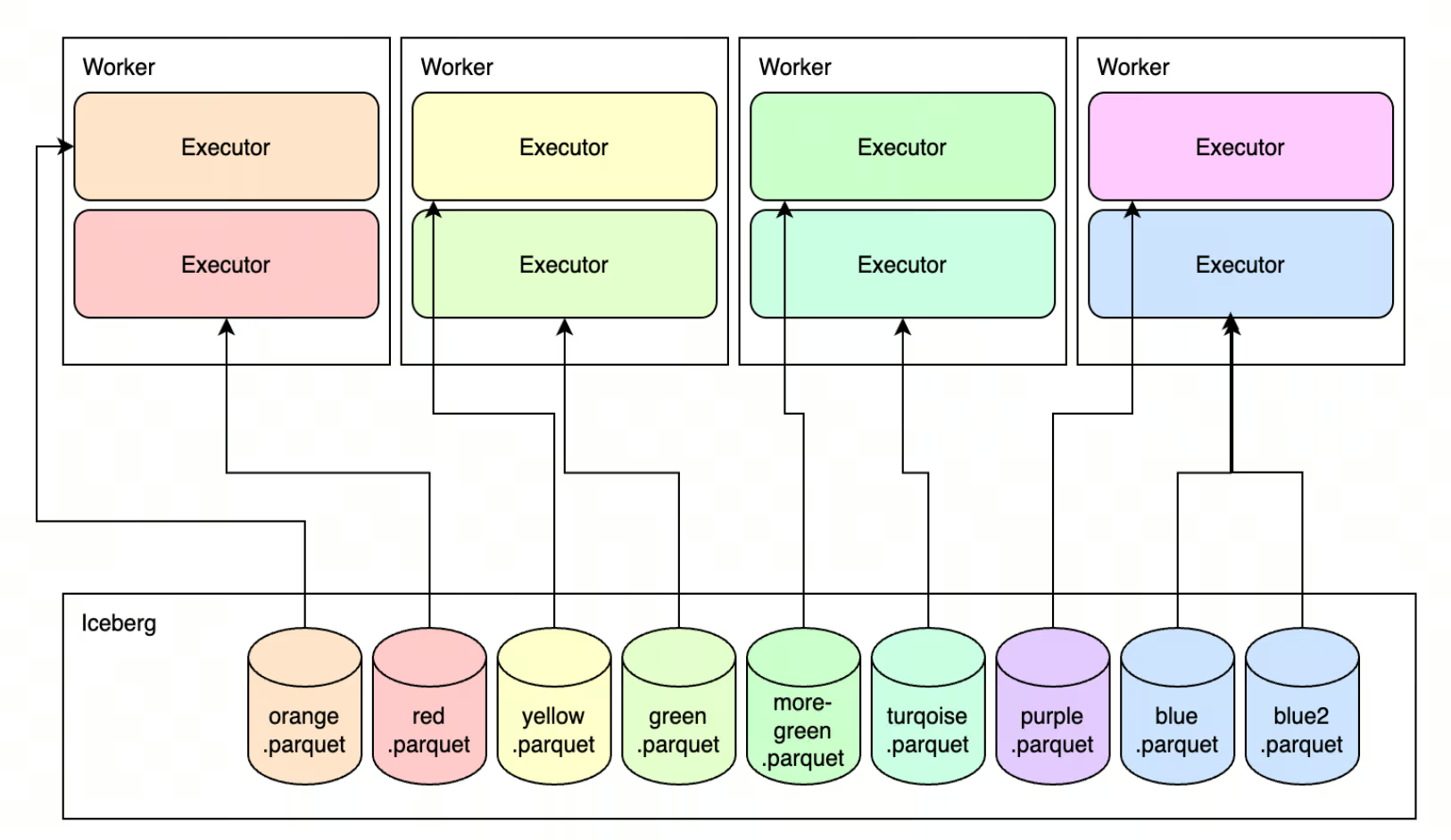
• The more modern approach is to rely on Apache Iceberg’s (or other V2 data sources like Delta, albeit with more limited support) partition-aware configurations. When data is written in Iceberg table and stored with a partition key, joining/aggregating on that partition key won’t require shuffle. However, applying this feature needs some configurations to be set (see bucketing in Iceberg, or StoragePartitionedJoin ), and ensure your Spark version supports such features (most bucketing related features are available from Spark 3.5.x and Spark 4.x).

Results

Note that the optimization above is done with vanilla Spark. We didn’t move to an accelerated Spark engine (like C++/Rust-based execution engine), but doing these improvements already significantly accelerated our Spark pipelines and cut costs at the same time.

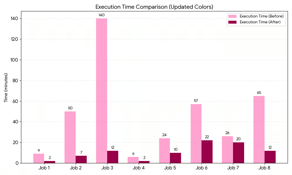
Across all the optimized jobs, the tricks outlined before generated ~76% in execution time savings, with ~63% cost reduction.